
Example Jupyter Notebook using the NVIDIA TensorFlow Container and the Fashion-MNIST data set
Fashion-MNIST Example with the NVIDIA TensorFlow Container from NGC
This notebook walks you through the basics of using containers from the NGC Catalog. We chose the GPU optimized TensorFlow container as an example, but the basics of working with docker containers apply to all NGC containers.
We will show you how to:
- Install the Docker Engine on your system
- Pull the TensorFlow container from the NGC Catalog using Docker
- Run the TensorFlow container using Docker
- Execute a simple image classification task using TensorFlow and Jupyter Notebook
Let's get started!
1. Install the Docker Engine
Go to https://docs.docker.com/engine/install/ to install the Docker Engine on your system.
2. Download the TensorFlow container from the NGC Catalog
Once the Docker Engine is installed on your machine, visit https://ngc.nvidia.com/catalog/containers and search for the TensorFlow container. Click on the TensorFlow card and copy the pull command.
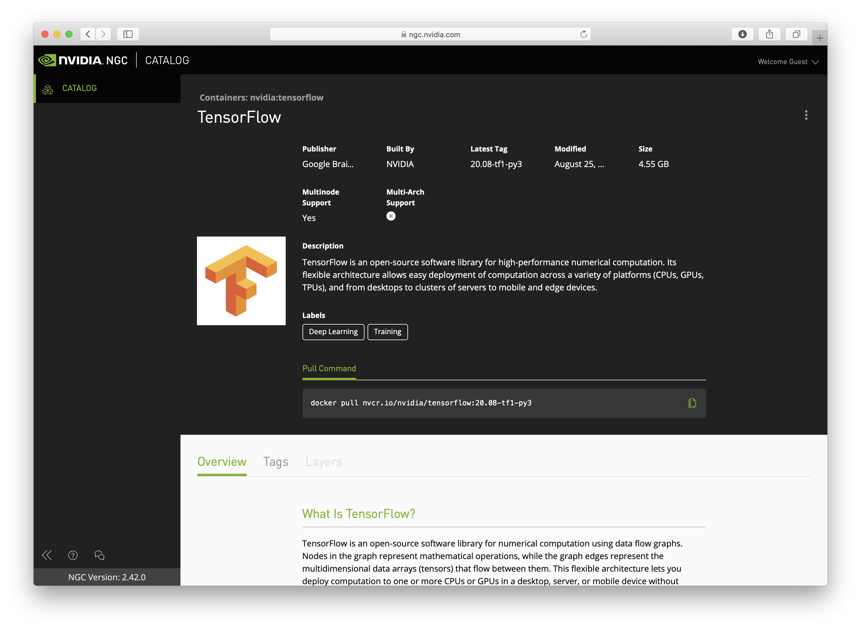
Open the command line of your machine and past the pull command into your command line. Execute the command to download the container.
$ docker pull nvcr.io/nvidia/tensorflow:20.08-tf1-py3
The container starts downloading to your computer. A container image consists of many layers; all of them need to be pulled.
3. Run the TensorFlow container image
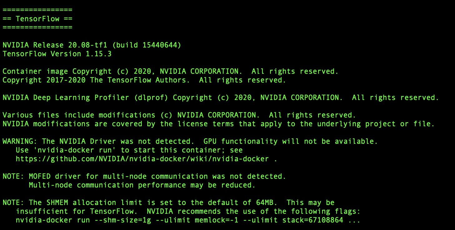
Once the container download is completed, run the following code in your command line to run and start the container:
$ docker run -it --gpus all -p 8888:8888 -v $PWD:/projects --network=host nvcr.io/nvidia/tensorflow:20.08-tf1-py3
4. Install Jupyter lab and open a notebook
Within the container, run the following commands:
pip install jupyterlab
jupyter lab --ip=0.0.0.0 --port=8888 --allow-root
Open up your favorite browser and enter: http://localhost:8888/?token=*yourtoken*.
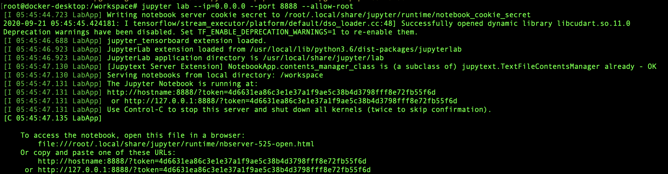
You should see the Jupyter Lab application. Click on the plus icon to launch a new Python 3 noteb ook.
Follow along with the image classification with the TensorFlow example provided below.
5. Fashion-MNIST Image Classification with TensorFlow
Follow the code to train a simple neural network that classifies images of clothing.
We are going to work with the Fashion-MNIST data set. The data set contains images of Zalando's article images. The images are divided into 10 classes, from 0 to 9, where each class represents a category of clothing:
| Class | Name |
|---|---|
| 0 | T-shirt/top |
| 1 | Trouser |
| 2 | Pullover |
| 3 | Dress |
| 4 | Coat |
| 5 | Sandal |
| 6 | Shirt |
| 7 | Sneaker |
| 8 | Bag |
| 9 | Ankle boot |
The Fashion-MNIST data set is part of the TensorFlow data set module.
Let's explore the data set:
There are 60000 images in the training set and 10000 images in the testing set.
There are 60000 labels in the training set and 10000 labels in the test set.
The images are 28 x 28 NumPy arrays.
array([9, 0, 0, 3, 0, 2, 7, 2, 5, 5, 0, 9, 5, 5, 7, 9, 1, 0, 6, 4],
      dtype=uint8)

Epoch 1/15
1875/1875 [==============================] - 1s 728us/step - loss: 0.4917 - accuracy: 0.8285
Epoch 2/15
1875/1875 [==============================] - 1s 672us/step - loss: 0.3757 - accuracy: 0.8652
Epoch 3/15
1875/1875 [==============================] - 1s 664us/step - loss: 0.3385 - accuracy: 0.8771
Epoch 4/15
1875/1875 [==============================] - 1s 669us/step - loss: 0.3144 - accuracy: 0.8847
Epoch 5/15
1875/1875 [==============================] - 1s 670us/step - loss: 0.2944 - accuracy: 0.8917
Epoch 6/15
1875/1875 [==============================] - 1s 662us/step - loss: 0.2805 - accuracy: 0.8964
Epoch 7/15
1875/1875 [==============================] - 1s 679us/step - loss: 0.2696 - accuracy: 0.8998
Epoch 8/15
1875/1875 [==============================] - 1s 675us/step - loss: 0.2566 - accuracy: 0.9053
Epoch 9/15
1875/1875 [==============================] - 1s 687us/step - loss: 0.2502 - accuracy: 0.9061
Epoch 10/15
1875/1875 [==============================] - 1s 664us/step - loss: 0.2406 - accuracy: 0.9107
Epoch 11/15
1875/1875 [==============================] - 1s 669us/step - loss: 0.2312 - accuracy: 0.9143
Epoch 12/15
1875/1875 [==============================] - 1s 666us/step - loss: 0.2230 - accuracy: 0.9170
Epoch 13/15
1875/1875 [==============================] - 1s 664us/step - loss: 0.2156 - accuracy: 0.9189
Epoch 14/15
1875/1875 [==============================] - 1s 671us/step - loss: 0.2106 - accuracy: 0.9206
Epoch 15/15
1875/1875 [==============================] - 1s 672us/step - loss: 0.2024 - accuracy: 0.9239
<tensorflow.python.keras.callbacks.History at 0x7fa10c1241d0>
With every epoch, the loss function decreases and the accuracy increases. After 15 epochs, the accuracy is around 92%.
313/313 [==============================] - 0s 542us/step - loss: 0.3482 - accuracy: 0.8836
The accuracy of the predictions is around 88%.
Here you go! You trained your first model and used it to make predictions on test data. For more advanced TensorFlow examples and in-depth explanations of the different steps, visit https://www.tensorflow.org/tutorials.
To explore all NGC Containers, visit https://ngc.nvidia.com/. The NGC Catalog offers not only GPU optimized containers but also Helm Charts, pre-trained models and model scripts.